Jump to a Section Below
Introduction |
Construction Dewatering (Solar) |
Ecological Resources (Solar) |
Stormwater Management
Decommissioning Summary (Solar) |
Renewable Portfolio (Solar) |
Greenhouse Gases |
Forest Conservation Act
Chesapeake Bay Critical Area Program |
Noise Impacts |
Climate Change (Solar) |
Maryland Agricultural Land Preservation Foundation (MALPF)
Maryland Heritage Areas Program |
Priority Preservation Area |
Priority Funding Areas |
Maryland's Rural Legacy Areas
Maryland’s Opportunity Zone Program |
Electromagnetic Field Impacts |
Fire Safety (Solar) |
Visual Impacts (Solar)
Property Values (Solar) |
Glare (Solar) |
Environmental Justice |
Cumulative Effects (Solar)
Soil Panel Leaching and Toxicity Concerns |
Electromagnetic Fields (Transmission)
Introduction
The Public Service Commission (PSC) is the regulating entity whose jurisdiction includes licensing power generating facilities and overhead transmission lines greater than 69 kilovolts (kV) within the state of Maryland. An applicant that is planning to construct or modify a generating facility or a transmission line must receive a permit, the Certificate of Public Convenience and Necessity (CPCN), from the PSC before the start of construction. As part of the licensing process, the Maryland Department of Natural Resources (DNR) Power Plant Research Program (PPRP), in coordination with other State agencies evaluates each facility’s potential impacts on environmental, socioeconomic, and cultural resources in Maryland, pursuant to Section 3-304 through 3-306 of the Natural Resources Article of the Annotated Code of Maryland (COMAR).
PPRP’s assessment is documented within a Project Assessment Report (PAR) for each individual power generating facility or overhead transmission line project. The following information is intended to provide general background information about some of the environmental, socioeconomic, and cultural program areas within Maryland and specific topics that are evaluated as part of PPRP’s assessment.
Sections below are marked as (Solar) to show content that relates specifically to solar photovoltaic (PV) power generation projects. All other content is applicable to any form of power generating facility as well as overhead transmission line projects.
Construction Dewatering (Solar)
Dewatering is a geotechnical process that involves the removal of groundwater from soil or rock in order to reduce the water content to a desired level. Dewatering is a crucial step in preparing an area for construction work.1 Code of Maryland Regulations (COMAR) section 20.79.03.02(B)(3)(c) requires an analysis of construction dewatering needs and calculations estimating amounts of water to be removed.
Groundwater
Groundwater is derived almost entirely from precipitation. It is the portion of the precipitation (rain or melting snow) that moves from the land surface into the soil by infiltration and then into underground storage and circulation. Of the water that falls on the land surface only about 25% enters the groundwater system. The direct surface runoff is the portion of precipitation which has not gone underground but runs over the surface as streams. Total runoff includes groundwater that discharges into streams, maintaining their baseflow.2
Underlying geology dictates the types and quality of the aquifers in each region. An aquifer is an underground reservoir that stores and yields groundwater in economically usable quantities. Estimated water levels throughout the state are tracked by the Maryland Geologic Survey
Groundwater Levels (MGS).
In general, west of the Fall Line which parallels Interstate 95, groundwater is found in fractures and bedding-plane partings in consolidated rock. Unconsolidated soils covers the rock in most places, and the water table may occur above or below the overburden-rock interface. Groundwater is generally found deeper within formations but may be found near the surface adjacent to ponds, streams, and wetlands.3
East of the Fall Line, the geologic units consist almost entirely of unconsolidated sediments overlying consolidated basement rock, and groundwater is found in void spaces between sand and gravel particles. Groundwater in this region is generally shallow.
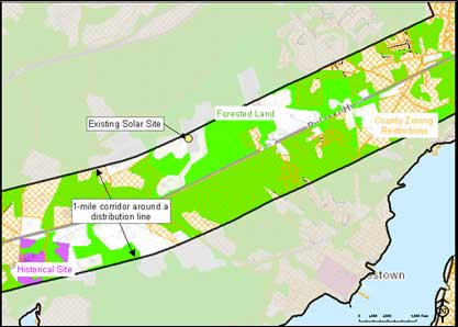
Fig. 1: Water cycle graphic showing groundwater fuction.
Permitting
Activities common to the construction of solar energy generating facilities such as utility trenching or installing footers may require dewatering if shallow groundwater is encountered. COMAR 26.17.06.03 requires all individuals or entities to obtain a permit from Maryland Department of the Environment (MDE) before appropriating or using waters of the State except for temporary dewatering4 during construction. Dewatering is considered temporary when the duration of the dewatering is expected to be less than 30 days; and the average water use does not exceed 10,000 gallons per day. However, for construction that will last longer than 30 days but use less than an annual average of 5,000 gallons/day, an applicant can qualify for a Water Appropriations Exemption. An applicant should assess dewatering needs for construction of the project prior to submitting their CPCN applications and determine whether a
Water Appropriation Permit or a
Water Appropriation Exemption Request is required. COMAR 20.79.03.02(B)(3)(i) requires an applicant to include the information and forms required by MDE relating to water use and appropriations under COMAR 26.17.06.07 and 26.17.07, if applicable, as part of any CPCN application.
Dewatering Guidance
The conditions at a particular site may necessitate the use of multiple dewatering practices to protect workers and structures. Water removed by pumps may require treatment to reduce turbidity prior to discharge to receiving waters.
Footnotes for this section:
Return to Top
Ecological Resources (Solar)
The web pages listed below are potential resources for CPCN Applications for solar photovoltaic (PV) facilities from Maryland Department of Natural Resources (DNR) and Maryland Department of the Environment (MDE). Direct, indirect, and cumulative effects of a project are assessed from the materials submitted by an applicant, along with other sources, and evaluated in PPRP’s Project Assessment Report (PAR).
Aquatic
Tier II Streams:
https://mde.maryland.gov/programs/water/tmdl/waterqualitystandards/pages/antidegradation_policy.aspx#:~:text=Tier%20II%2C%20high%20quality%2C%20waters,specified%20in%20water%20quality%20standards.
Wild and Scenic Rivers:
https://dnr.maryland.gov/land/pages/stewardship/scenic-and-wild-rivers.aspx
Terrestrial
Wetlands of Special State Concern:
https://mde.maryland.gov/programs/water/WetlandsandWaterways/DocumentsandInformation/Documents/www.mde.state.md.us/assets/document/WetlandsWaterways/ssc.pdf
Vegetation
Forest Interior Dwelling Species (FIDS):
https://mde.maryland.gov/programs/Water/WetlandsandWaterways/Documents/Solar/Conservation_Forest_dwelling_birds_2000.pdf
https://dnr.maryland.gov/land/Pages/Green-Infrastructure-Forests.aspx
Green Infrastructure:
https://dnr.maryland.gov/land/Pages/Green-Infrastructure.aspx
https://dnr.maryland.gov/land/Pages/Green-Infrastructure-Mapping.aspx
Wildlife
Biodiversity Conservation Network (BioNet):
https://dnr.maryland.gov/wildlife/Documents/BIONET_FactSheet.pdf
Invasive Species:
https://dnr.maryland.gov/Invasives/pages/default.aspx
https://dnr.maryland.gov/forests/pages/programapps/pests.aspx
Spotted Lanternfly:
https://mda.maryland.gov/plants-pests/Pages/spotted-lantern-fly.aspx
The Spotted Lanternfly Quarantine Order seeks to prevent the spread of Spotted Lanternfly in the State by setting in place a permitting process to control the movement of vehicles and materials that could transport the species to new locations. Potential invasion modes include transporting any of several dozen items across county/state lines (including mulch, any tree parts, firewood, nursery stock, decorative stone, and any outdoor household equipment such as lawnmowers). It also establishes decontamination protocols for construction materials, equipment, and personnel working in or coming from a quarantine area.
Rare, Threatened, or Endangered (RTE) Species:
https://dnr.maryland.gov/wildlife/Pages/plants_wildlife/rte/espaa.aspx
https://dnr.maryland.gov/wildlife/Pages/plants_wildlife/rte/rteanimals.aspx
Sensitive Species Project Review Areas (SSPRAs):
https://dnr.maryland.gov/wildlife/pages/plants_wildlife/sspra.aspx
Wildlife Management Areas:
https://dnr.maryland.gov/wildlife/Pages/publiclands/home.aspx
Footnotes for this section:
1Maryland Division of State Documents. Maryland.gov Enterprise Agency Template. (n.d.).
https://dsd.maryland.gov/regulations/Pages/20.79.03.02.aspx
Return to Top
Stormwater Management
The State of Maryland has comprehensive programs for stormwater management and erosion and sediment control, to reduce adverse impacts of development on streams and wetlands and improve water quality. These requirements address both the temporary and the permanent impacts associated with development activities.
An Applicant must comply with:
- COMAR 26.17.01 and COMAR 26.17.02 - the preparation, submittal, review, approval, and enforcement of erosion, sediment and stormwater control plans, including any dewatering plans;
- COMAR 26.08.01 through 26.08.04 - regulates discharges to waters of the State and maintenance of surface water quality; and
- the Maryland Stormwater Design Manual, Volumes I and II with Supplement No. 1, and Technical Memo #8 dated March 30, 2018 (or updated guidance) - the official guide for stormwater management principles, methods, and practices in Maryland
1.
Applicable Definitions:
- Best Management Practice (BMP): “conservation practices and management measures that control soil loss and reduce water quality degradation caused by nutrients, animal wastes, toxics, and sediment.”2
- Environmental Site Design (ESD): “using small-scale stormwater management practices, nonstructural techniques, and better site planning to mimic natural hydrologic runoff characteristics and minimize the impact of land development on water resources.”3
- Grad(ing): “to disturb earth by, including but not limited to, any excavation, filling, stockpiling, grubbing, removing root mat or topsoil, or any combination thereof."4
- Impervious Surface: “A surface which does not allow water or other liquids to pass through. Impervious surfaces increase the volume and velocity of runoff and the amount of pollution and sediment that enters streams and lakes.”5
- Non-rooftop Disconnection: “the process of directing flow from impervious surfaces onto vegetated areas where it can soak into or filter over the ground.”6
- Soil Compaction: “occurs when soil particles are pressed together, reducing pore space between them. Heavily compacted soils contain few large pores, less total pore volume and a greater density. Compacted soil has reduced water infiltration and drainage, because large pores more effectively move water downward through the soil than smaller pores.”7
Grading is often needed for installing concrete pads, foundations, and access roads. This practice results in soil compaction in the areas where heavy machinery rolls over the ground. In addition to the soil compaction from construction equipment and access roads, the concrete pads, racking posts (for solar facilities), and entrance improvements will reduce the area available for water infiltration.
Impervious surfaces also decrease the amount of stormwater that can infiltrate the ground, increasing the amount of stormwater runoff. This can affect streams and wetlands by increasing sediments and introducing any contaminants that were on the impervious surfaces, such as oil from construction vehicles, into the nearest waterbody. These practices, while increasing runoff to nearby streams, also result in root growth and plant establishment issues, drowned roots, root rot, and increased soil acidity.8
Slope also directs where stormwater flows from a project site. Areas with gentle slopes slow the runoff allowing for water infiltration. Areas with steeper slopes have runoff that flows faster towards an area with the lowest topography, usually a stream or river in the area. If water reaches streams too quickly, the fast-moving water can increase streambank erosion and lead to flooding.
An applicant is required to obtain a National Pollutant Discharge Elimination System (NPDES) General Permit for construction activities over one acre, as well as an Erosion and Sediment Control and Stormwater Management Plan. Achieving effective stormwater infiltration for the completed facility may be dependent on avoiding soil compaction during construction or re- loosening compacted areas before planting the cover grass.
During construction when there is potential for stormwater runoff to affect nearby streams and wetlands, a third-party monitor is often beneficial to observe the stormwater management process and ensure that the correct mitigation measures are being taken.
Specific to solar facilities, where the slopes are less than 10 percent, non-rooftop disconnection credits can be used in accordance with MDE’s 2013 white paper entitled “Stormwater Design Guidance – Solar Panel Installations.”9 With slopes between 0 and 5 percent, no additional practices are necessary, as the practice of non-rooftop disconnection is enough to redirect runoff from entering a nearby waterbody. However, in areas between 5 and 10 percent, other BMPs, such as level spreaders that reduce concentrated flow and improve infiltration, will need to be utilized to help redirect the runoff.
The soil in some areas may become compacted from any grading activities and heavy equipment traffic in staging areas or construction areas. If the resulting soil compaction is on the areas to be used for “Non-Rooftop Disconnected Impervious Area” crediting, it will void the intended benefit. Recent work10,11,12 shows that soil decompaction and amendment can be highly effective at improving stormwater infiltration and providing deeper, longer water storage after such compaction. Therefore, to ensure proper post-construction runoff characteristics and planting success, ripping (mechanically breaking up compacted soil) can be performed to a minimum depth of 12 inches and compost amendment in all compacted areas (e.g., graded areas, staging areas, or heavily trafficked areas) that will be included in a Non-Rooftop Disconnection Credit area.
Potential Mitigation Practices
Mitigation factors to aid in managing the stormwater that enters streams near a given solar facility are as follows:
- Grading and Stormwater Management
- Designing any grading and associated stormwater controls to minimize hydrological changes to streams and wetlands.
- Designing controls to maintain the existing flow regime to streams and wetlands.
- Sediment Control
- Requiring an applicant to submit an Erosion and Sediment Control Plan to the applicable county for review and approval before construction.
Footnotes for this section:
1 Maryland Stormwater Design Manual, Maryland.gov, May,2009.
https://mde.maryland.gov/programs/water/stormwatermanagementprogram/pages/stormwater_design.aspx
2 Glossary of Terms, Maryland Department of Natural Resources.
https://dnr.maryland.gov/criticalarea/pages/glossary.aspx#i
3 Environment Article, Title 4, Subtitle 2 Stormwater Management, Annotated Code of Maryland.
https://advance.lexis.com/container?config=00JAA1NTM5MzBmZC02MTg2LTQzNmEtYmI5Yy0yZWEwYzA1OGEwNTYKAFBvZENhdGFsb2fdgr2eooaZj7MpSZGOIwWq&crid=8d9e4041-43aa-4d70-8f00-804698c701a9&prid=1c108f55-e0b2-4646-9c80-3940ceb97d88
4 2011 Maryland Standards and Specifications For Soil Erosion and Sediment Control, ACKNOWLEDGEMENTS, Maryland Department of the Environment, et.al, Dec, 2011.
https://mde.maryland.gov/programs/water/StormwaterManagementProgram/Documents/2011%20MD%20Standard%20and%20Specifications%20for%20Soil%20Erosion%20and%20Sediment%20Control.pdf
5 MDE Glossary of Terms, Maryland Department of the Environment.
https://mde.maryland.gov/Documents/MDE-Glossary.pdf
6 Maryland Stormwater Design Manual, Volumes 1 and 2, Chapter 5 Environmental Site Design, Maryland Department of the Environment, 2009.
https://mde.maryland.gov/programs/water/StormwaterManagementProgram/Documents/www.mde.state.md.us/assets/document/Design%20Manual%20Chapter%205%2003%2024%202009.pdf
7 DeJong-Hughes, J, Soil compaction, UMN Extension, 2018.
https://extension.umn.edu/soil-management-and-health/soil-compaction#sources-1200560
8 Common Soil Problems, University of Maryland Extension, Feb 17, 2023.
https://extension.umd.edu/resource/common-soil-problems/
9 ESDMEP Design Guidance – Solar Panel Installations, Maryland Department of the Environment.
https://mde.maryland.gov/programs/water/StormwaterManagementProgram/Documents/ESDMEP%20Design%20Guidance%20Solar%20Panels.pdf
10 Haynes, Matthew A., Richard A. McLaughlin, and Joshua L. Heitman. 2013. "Comparison of methods to remediate compacted soils for infiltration and vegetative establishment."
Open Journal of Soil Science 3.05 (2013): 225;
11 Schwartz, Stuart S., and Brennan Smith. “Restoring hydrological function in urban landscapes with suburban subsoiling.”
Journal of Hydrology 543 (2016): 770-781; SHA 2016.
12 Schwartz, Stuart S., and Brennan Smith. “Sustainable Landscaping Practices for Enhancing Vegetation Establishment.”
Maryland State Highway Administration Research Report MD-16-SHA/UMBC/1-1. (2016).
Return to Top
Decommissioning Summary (Solar)
In general, the developers of solar photovoltaic (PV) facilities design their projects for a finite operating life span. Although as of 2024, no solar facilities have yet been decommissioned in Maryland, planning for decommissioning is a common practice across the solar power industry. Solar facilities operating under CPCN authority must have a robust decommissioning plan in place to ensure that future landowners can use the parcels in a manner that is not hindered by their former use for solar generation and the cost of decommissioning is not borne by the State, county, or municipal authority.
A solar facility decommissioning plan describes the responsible party(ies), timeframes, expected sequence of activities, and estimated costs for decommissioning, dismantling, legal disposal of all components, and restoration of the affected land. At the time of decommissioning, an applicant must prepare a final plan that reflects the actual intended land use and complies with regulations and standards that are in place at that time. The final decommissioning plan will be reviewed and approved by local and State authorities as required prior to the start of decommissioning activities.
The plan must include an estimate of decommissioning costs, prepared by a knowledgeable third party, addressing the safe removal and proper disposal of all components of a project. These components include, but are not limited to, solar panels, cables, wires, steel racks, and above and below ground foundations. If salvage value is to be included in the decommissioning cost, an applicant must provide reliable documentation to support its cost estimate. The applicant must also show that they are maximizing, to the extent possible, recycling and reuse of facility components.
To ensure that decommissioning costs are not borne by the State, county, or other municipal authority at the end of the useful life of a project or in the event of abandonment of a project, an applicant must also secure a funding mechanism(s) to cover the cost of implementing the decommissioning plan. The financial instrument may be in the form of a surety bond, a letter of credit issued by a financial institution, insurance, trust fund, sinking fund, or land-lease arrangement. A facility will be considered abandoned if there is no output from the project to the grid for a period of 12 consecutive months.
Within five years after a CPCN is granted, and every five years thereafter, solar facility owners must revise the decommissioning plan, cost estimate, and financial assurance mechanism to adjust for inflation, to reflect the ongoing evolution of the recycling and resale markets for solar panels, and to incorporate any other necessary changes.
For guidance purposes, the topics to be addressed in a solar decommissioning plan are outlined below.
- Party(ies) responsible for decommissioning activities
- Time required to accomplish decommissioning
- Anticipated schedule
- Criteria that would trigger decommissioning
Activities associated with dismantling and removing/disposing of all components, including cables, wiring, and foundations
- below and above ground
- Maximizing the extent of component recycling and reuse, where practicable
- Materials handling in accordance with applicable federal, State, county and local requirements
- Stabilization, grading and seeding all disturbed areas
- Distribution of topsoil stockpiled on site
- Financial instrument specified
In addition, the solar decommissioning cost estimate should address the following items.
- Prepared by third party consultant
- Costs broken down by task or activity
- Tasks/activities are consistent with narrative description of planned decommissioning activities
- Transportation costs included for disposal/recycling
- Safe removal and proper disposal of components containing hazardous materials
- Unit costs identified
- Detailed costing assumptions clearly identified
- Documentation of salvage value (if included in the cost estimate)
- Proposed value for financial surety
Return to Top
Renewable Portfolio (Solar)
Under COMAR 20.79.03.02 B(6)(a), applicants are required to include a discussion of the impact of a proposed generation project to satisfy the requirements of the Maryland Renewable Portfolio Standard (RPS), if applicable. The Maryland RPS requires electricity suppliers to demonstrate annually that a certain percentage of electricity sales are satisfied with generation from eligible renewable energy technologies. For 2024, electricity suppliers must have 36.2% of its electricity sales from eligible renewable energy technologies, of which 6.5% must come from solar generation facilities that are connected to the utility distribution grid serving state electricity customers. These requirements increase annually to 2030, where 52.5% of an electricity supplier’s sales must come from eligible renewable energy technologies, 14.5% of which must come from solar.
Return to Top
Greenhouse Gases
Greenhouse gases (GHG) are gases that trap heat in the atmosphere. Carbon dioxide (CO2) is the primary GHG emitted through human activities, such as burning fossil fuels, (i.e., coal, natural gas, and oil). Other types of greenhouse gases associated with human activities are methane (CH4), nitrous oxide (N2O), and fluorinated gases (e.g., hydrofluorocarbons [HFCs], perfluorocarbons [PFCs], and sulfur hexafluoride [SF6]). Under COMAR 20.79.03.02 B(6)(b) power generators are required to include in their environmental review document the impact of the proposed facility or modification to the greenhouse gas (GHG) reduction requirements set forth in Environment Article, §2-1201, et seq., Annotated Code of Maryland.
PPRP uses the EPA’s Avoided Emissions and Generation Tool (AVERT) tool to evaluate the impact of a renewable energy project to Maryland’s GHG reduction requirements.1 AVERT is a free tool designed to evaluate the county, state, and regional changes in CO2 and several other greenhouse gases from electric power plants and displaced fuel-burning vehicles resulting from energy policies and programs such as energy efficiency, renewable energy, and electric vehicles. Specifically, AVERT allows users to estimate the yearly avoided GHG emissions associated with the operation of solar photovoltaic and wind projects. A limitation of AVERT is its inability to predict emissions beyond five years.
Footnote for this section:
Return to Top
Forest Conservation Act
In 2013, the General Assembly established that it is the policy of the State to achieve no net loss of forest1 not just in extent, but also in terms of quality.
The term "no net loss of forest" means that 40 percent of all land in Maryland is covered by tree canopy.2 That is, the statewide total of forest losses and gains must be balanced to maintain the 40 percent cover objective. The Sustainable Forestry Council adopted a green infrastructure approach and prioritized protection of high-quality forests and created a strategy to mitigate loss. The Forest Conservation Act (FCA)3 provides the mechanism for distributing those losses and gains among development projects to achieve the net balance. An individual project is not evaluated directly against the no net loss standard.
The FCA applies two tests to determine the amount of forest cover that a project must establish, replant, or retain to contribute to the statewide no net loss goal:
-
Afforestation Threshold: based on a minimum forest cover percentage for each land use type. Post construction, the FCA requires that the project meet the Afforestation Threshold (preferably on-site) even if no trees are cut or removed.
-
Forest Conservation Threshold (Reforestation): replacing any existing trees/forest that are removed for the project, either on the development site or at another acceptable location.
Forest losses between the Afforestation Threshold and the Forest Conservation Threshold (an equal or higher forest cover percentage) require a 2:1 replacement, while losses above the Forest Conservation Threshold may be replaced at a lower (1:4) ratio.4
The FCA establishes specific minimum forest cover thresholds for land development that make the identification and protection of forests and other sensitive areas an integral part of the site planning process. Depending on the land use type, zoning, initial forest cover of a project site, and the amount of forest retained, some projects will contribute more than the no net loss 40 percent cover percentage and some less. The State achieves the overall statewide goal of 40 percent forest cover using both afforestation and replacement/reforestation rules across many projects; the "no-net-loss" policy cannot be applied on an individual project basis.
In general, county and municipal governments are responsible for making sure that the State's Forest Conservation standards are met through local ordinances but may choose to implement more stringent criteria than required by the FCA. In CPCN cases, however, Section 5-1603(f) of the Natural Resources Article instructs the PSC to make an appropriate determination about afforestation and reforestation under the provisions of the State FCA:
After December 31, 1992, the Public Service Commission shall give due consideration to the need to minimize the loss of forest and the provisions for afforestation and reforestation set forth in this subtitle together with all applicable electrical safety codes, when reviewing applications for a certificate of public convenience and necessity issued pursuant to § 7–204, § 7–205, § 7–207, or § 7–208 of the Public Utilities Article.
Through this process, the PSC can give the appropriate weight to state forest conservation policies and regulations, local jurisdictional preferences, and the specialized nature of electrical power facilities in determining the developer's FCA obligations.
The FCA also specifies that high-priority areas for afforestation or reforestation include establishing or enhancing buffers adjacent to intermittent or perennial streams, establishing or increasing forest corridors, and establishing or enhancing forest buffers adjacent to critical habitats or on 100-year floodplains.5 PPRP encourages applicants to design its landscape buffers, or perhaps expand them slightly, to achieve one or more of these goals.
Per COMAR 20.79.03.03 (B)(1), an applicant shall include the following in its environmental review document:
- A forest stand delineation.
- Any techniques used to minimize forest impact.
- A proposal to address applicable forest conservation ordinance of the county or municipality in which any portion of the project is to be located.
Specific to solar facilities, landscape buffers, vegetation planted along the edge of a parcel that is used to screen the facility to reduce visibility, are often required by counties or municipalities. In certain cases, a landscape buffer can be used to contribute to the FCA mitigation requirement. PPRP can accept this approach as long as the landscape buffer plantings include contiguous areas that meet the definition of forest in Natural Resources Article 5-1601(k):
- “Forest” means a biological community dominated by trees and other woody plants covering a land area of 10,000 square feet or greater.
- “Forest” includes:
- Areas that have at least 100 trees per acre with at least 50% of those trees having a 2-inch or greater diameter at 4.5 feet above the ground; and
- Forest areas that have been cut but not cleared.
- “Forest” does not include orchards.
PPRP notes that Maryland Governor Wes Moore signed House Bill 723 in May 2023, which serves as an amendment to the Forest Conservation Act. The changes reflected in this legislation will go into effect on July 1, 2024.
Footnotes for this section:
Return to Top
Chesapeake Bay Critical Area Program
The Chesapeake Bay Critical Area (CBCA) Program regulates and restricts land development within 1,000 feet of tidal waters and tidal wetlands of the Chesapeake Bay, Atlantic Coastal Bays, and their tributaries under Title 27 of COMAR.1 The CBCA Program was created by the passage of the Critical Area Act by the Maryland General Assembly in 1984. Local governments implement the CBCA Program. However, the Critical Area Commission (CAC), a statewide entity formed by the Critical Area Act of 1984, oversees the actions of local governments. The CAC has designed a set of standards, or Critical Area Criteria, which are then adopted into local ordinances that govern land use and development.1 While individual local governments typically make decisions on development proposals, the state CAC has the authority to review and comment on them. Critical Area restrictions overlay normal zoning regulations and are applied in addition to them.
The CBCA includes three types of management areas, each of which allow different uses:
-
Intensely Developed Area (IDA) – IDAs are areas with the least restrictive land-use classification, are designated for high-intensity development. They are defined as areas of twenty or more adjacent acres where residential, commercial, institutional, or industrial land uses predominate.
-
Limited Development Area (LDA) – LDAs are areas with the middle land-use classification and are designated for moderate intensity residential development and limited commercial development. While LDAs are not dominated by open space, they must conserve existing areas of natural habitat and incorporate wildlife corridors that ensure continuity of wildlife and plant habitat. Housing densities in LDAs are based on local zoning regulations.
-
Resource Conservation Area (RCA) - RCAs are the most restrictive land-use classification, and are designated for resource protection or utilization, as well as low-intensity residential development. RCAs are characterized by natural environments or by resource-based activities such as agriculture, aquaculture, commercial forestry, or fishing.
The Critical Area Buffer, which lies within 100 feet of tidal waters, wetlands and tributary streams, and Habitat Protection Areas, was established as a protective buffer around aquatic resources within the Critical Area. No development activities are permitted within the 100-foot buffer except those associated with water dependent facilities and those which have obtained a variance through the local government.
Footnotes for this section:
Return to Top
Noise Impacts
Definition of Noise
Noise generally consists of many frequency constituents of varying loudness. Three decibels (dB) is approximately the smallest change in sound intensity that can be detected by the human ear. A tenfold increase in the intensity of sound is expressed by an additional 10 units on the dB scale, a 100-fold increase by an additional 20 dB. Because the sensitivity of the human ear varies according to the frequency of sound, a weighted noise scale is used to determine the impacts of noise on humans. This A-weighted decibel (dBA) scale weights the various components of noise based on the response of the human ear. For example, the ear perceives middle frequencies better than low or very high frequencies; therefore, noise composed predominantly of the middle frequencies is assigned a higher loudness value on the dBA scale. Subjectively, a tenfold increase in sound intensity (10 dB increase) is perceived as an approximate doubling of sound. Typical A-weighted sound levels for various noise sources are shown in the table below.
Typical Sound Levels for Common Sources (dBA)
| Noise Source | Typical Sound Pressure Level |
|---|
| Lowest sound audible to human ear | 10 |
| Soft whisper in a quiet library | 30-40 |
| Light traffic, refrigerator motor, gentle breeze | 50 |
| Air conditioner at 6 meters, conversation | 60 |
| Busy traffic, noisy restaurant, freight train moving 30 mph at 30 meters | 70 |
| Subway, heavy city traffic, factory noise | 80 |
| Truck traffic, boiler room, lawnmower | 90 |
| Chain saw, pneumatic drill | 100 |
| Rock concert in front of speakers, sand blasting, thunder clap | 120 |
| Gunshot, jet plane | 140 |
Sound energy dissipates with increasing distance from the noise source. For every doubling of the distance, the sound pressure level produced by a given noise source decreases by approximately 6 dBA.
Summary of Regulatory Requirements
Maryland noise regulations specify maximum allowable noise levels, which are shown in the Table below (COMAR 26.02.03). The maximum allowable noise levels specified in the regulations vary with zoning designation and time of day. The noise limit for residential areas is 55 dBA during nighttime hours and 65 dBA during daytime hours. A noise source may not create noise that exceeds the allowable levels, as measured at the receiving property.
Maximum Allowable Noise Levels (dBA) for Receiving Land Use Categories1
| Zoning Designation |
| Industrial | Commercial | Residential |
|---|
| Day | 75 | 67 | 65 |
| Night | 75 | 62 | 55 |
Note: Day refers to the hours between 7 AM and 10 PM; night refers to the hours between 10 PM and 7 AM.
The State regulations exempt certain noise sources and noise-generating activities. For example, motor vehicles on public roads are exempt from Maryland noise regulations; however, while on industrial property, trucks are considered part of the industrial source and are regulated as such. The regulations also allow for construction activity to generate noise levels up to 90 dBA during daytime hours, but the nighttime standard may not be exceeded during construction.
While the State has established target levels for noise, enforcement authority for noise regulations rests with the local government.
Solar (Photovoltaic) Project Noise Impacts
Operational noise from solar photovoltaic (PV) facilities is typically low. The PV panels and support equipment do generate some noise, primarily associated with the power inverters and electrical transformers. Regarding noise generated by the power inverters and electrical transformers, a study conducted for the Massachusetts Clean Energy Center (2012)2 found that operational noise is inaudible at moderate distances. The measured noise levels from the PV arrays included in the study declined to ambient background noise levels at distances between 50 and 150 feet.
Some projects may include tracking mechanisms which change the angle of the panels for maximized generation. While there is some audible noise associated with the motors in the solar panel tracking mechanism, a 2013 report from Argonne National Laboratory concluded that such mechanical noise was not a significant source of noise for off-site receptors3.
Footnotes for this section:
1 COMAR 26.02.03.02, Environmental Noise Standards
https://dsd.maryland.gov/regulations/Pages/26.02.03.02.aspx
2 Massachusetts Clean Energy Center 2012. Study of Acoustic and EMF Levels from Solar Photovoltaic Projects. Prepared by Tech Environmental, Inc., Waltham, MA, for Massachusetts Clean Energy Center. December 17, 2012.
https://files.masscec.com/research/StudyAcousticEMFLevelsSolarPhotovoltaicProjects.pdf
3 ANL 2013, An Overview of Potential Environmental, Cultural, and Socioeconomic Impacts and Mitigation Measures for Utility-Scale Solar Energy Development, Environmental Science Division, Argonne National Laboratory, ANL/EVS/R-13/5. June 18, 2013.
https://www.researchgate.net/publication/320944992_An_Overview_of_Potential_Environmental_Cultural_and_Socioeconomic_Impacts_and_Mitigation_Measures_for_Utility-Scale_Solar_Energy_Development
Return to Top
Climate Change (Solar)
Public Utilities Article Section 7-207(e)(3) requires the PSC to consider how climate change will affect generation stations.
For proposed generation facilities, both the potential contribution of the facility to climate change and the potential effects of climate change on the facility must be evaluated. Potential changes in Maryland's climate during the lifetime of a solar photovoltaic facility (roughly 35 years) include:
- Sea level rise - an increase in mean sea level relative to a point on land;1
- Higher average and extreme air temperature (1 to 2 degrees Celsius) and more extreme temperature days per year; and
- An increase in the frequency or intensity of severe storms.
Sea Level Rise
COMAR 20.79.03.03(B)(8) requires an applicant to identify sea level rise areas in their environmental review document. Sea level rise could cause an increase in the occurrence of flooding, specifically on flat low-lying solar facilities, often occurring in Maryland’s Eastern Shore, and coastal areas along the Chesapeake Bay and the Atlantic Ocean. While it is less likely, effects from sea level rise could also be seen in solar facilities adjacent to rivers that are direct tributaries to the Chesapeake Bay and Atlantic Ocean. Flooding that short circuits electrical components (e.g., panels, transformers, inverters, power cables, etc.) could result in fire or destructive power surges in these components. High levels of damage or catastrophic destruction would likely result in cleaning up and rebuilding the facility, or complete decommissioning.

Sea Level Rise of Chesapeake Bay 2
Temperature
Warmer average and extreme high temperatures could augment the heating effect of the panels, transformers, and inverters. Solar panels change the absorption, reflection, conversion, and emission of solar energy to nearby land surfaces compared to either bare ground or vegetation. The “land surface energy balance” that results from these factors depends on the topography and soil moisture of the land surface, as well as the vegetation or materials that cover it. Solar panels convert approximately 20 percent of the incoming solar radiation to usable electricity while vegetation only uses about 2 percent for photosynthesis. On the other hand, solar facilities must re-radiate excess heat directly to the air while vegetation uses the excess energy to move and evaporate soil water into the atmosphere (evapotranspiration). These differences can be quantified by measuring the components of the energy flows.
Land surface energy balance, and the resulting fluxes of heat and water, are well-studied for vegetated areas,3 but less effort has been devoted to measuring the fluxes at solar facilities. There have been reported observations4 of wind, temperature, solar irradiance, relative humidity, and rainfall in and near a solar facility. They found that annual average temperatures above the solar panels were slightly higher than areas without solar panels (1.9 degrees Celsius), with above-ambient temperatures occurring during the day and below-ambient temperatures at night. This heat effect dissipated rapidly in the vertical direction (within 5 to 20 meters) and decreased gradually in the horizontal direction (within 300 meters). The authors indicated that these differences were insufficient to cause adverse micro-climate changes but did not assess the potential biological effects. Climate change studies have indicated that for some species, temperature-dependent growth processes such as the timing of spring leaf-out or flowering can be shifted by days or weeks by increases or decreases in the average temperature of this magnitude.5
Another study found, however, that the surface below solar photovoltaic (PV) panels remained cooler during the day and warmer at night than exposed surfaces.6 In former farm fields, such diurnal differences could reduce soil water evaporation and enhance growing conditions for grasses below the panels, depending on the panel configuration. A National Renewable Energy Laboratory study7 found that vegetation growth below sun-tracking panels was different on the east and west sides of the panels. This variance was attributed to consistent time-of-day differences in shading and precipitation runoff: clouds and rain events occurred primarily in the afternoon in their test area, while mornings were predominantly sunny and dry.
Although the heating effect of the panels and potential climate warming effects are each only on the order of 1 to 2 degrees, these small changes may affect pollinators and flower availability or other wildlife that depend on these plants and change their behavior or the general composition of the ecosystem within the facility fence. Whether these local changes will be positive or negative is currently hard to predict, and areas beyond the facility boundaries will respond only to any general climate-induced component of the temperature changes.
Severe Storms
Maryland’s Eastern Shore has historically been subjected to hurricanes. According to the Maryland State Archives website,8 a Category 3 (winds above 111 miles per hour [mph]) or higher hurricane has never hit the state of Maryland, but high winds and heavy rains from Category 1 and/or 2 hurricanes have caused damage (hurricane classification for older storms is approximate). Maryland experienced direct hits from hurricanes in 1878 and 1933, while in 2011 hurricane-force winds from Hurricane Irene (Category 1, winds 74 to 95 mph) affected some counties on the Delmarva Peninsula. The winds and rain associated with the storm caused power outages and flooding. The Archives website also notes that Maryland averages three tornadoes per year, with the most powerful (in 2002) reaching wind speeds of 260 mph (level 5 on the Fujita scale).
Based on climate change models, the general expectation is that events similar to such past events may occur more frequently, or that storms that occur may be stronger (higher winds) or more intense (more rainfall). Thus, past events can be used as a guide to prepare for potential future storms, but it should be kept in mind that predicting future storm tracks or intensities is beyond the capabilities of global circulation models, with or without accounting for potential climate change. In other words, there is no scientific way to state when or if a future hurricane or tornado will affect a proposed solar facility on the eastern shore.
Nonetheless, it must be recognized that future storms of this magnitude are likely to affect the State and could be accompanied by severe winds and flooding. Recent severe storms in other areas have illustrated the potential for massive destruction of solar facilities because wind forces produced in hurricanes and tornadoes are capable of exceeding the maximum ratings of racking systems and panels. Storm-caused flooding could inundate components of solar facilities as well, especially in the flat low-lying areas of a facility site.

Hurricane Storm Surge of the Chesapeake Bay 9
Footnotes for this section:
1 Sea Level Rise, University of Maryland Extension.
https://extension.umd.edu/programs/environment-natural-resources/program-areas/coastal-climate-program/sea-level-rise/
2 Data used in this figure comes from Maryland’s Environmental Resources and Land Information Network (MERLIN).
https://maryland.maps.arcgis.com/apps/webappviewer/index.html?id=434b195197364344a661da85c9bab3c9
3 Sellers, P.J., M.D. Heiser, F.G. Hall, S.J. Goetz, D.E. Strebel, S.B. Verma, R.L. Desjardins, P.M. Schuepp, and J.I. MacPherson. 1995.
"Effects of Spatial Variability in Topography, Vegetation Cover, and Soil Moisture on Area-Averaged Surface Fluxes: A Case Study using the FIFE 1989 data." J. Geophys. Research, Vol. 100, No. 012, pp. 25,607- 25,629.
4 Fthenakis, Vasilis and Yuanhao Yu. 2013. "Analysis of the Potential for a Heat Island Effect in Large Solar Farms."
Proc. 39th IEEE Photovoltaic Specialists Conference. June 16-21, 2013. Pages 3362-3366.
5 Song, Y., Zajic, C. J., Hwang, T., Hakkenberg, C. R., & Zhu, K. (2021).
Widespread mismatch between phenology and climate in human-dominated landscapes. AGU Advances, 2, e2021AV000431.
https://doi.org/10.1029/2021AV000431
6 Dominguez, Anthony, Jan Kleissl, and Jeffrey C. Luvall. 2011. "Effects of Solar Photovoltaic Panels on Roof Heat Transfer".
Solar Energy, Vol. 85, No. 9, pp. 2244-2255.
7 NREL 2017. Native Vegetation Performance under a Solar PV Array at the National Wind Technology Center. NREL Technical Report TP-1900-66218 prepared by Brenda Beatty, Jordan Macknick, James McCall, and Genevieve Braus, National Renewable Energy Laboratory, and David Buckner ESCO Associates Inc. May 2017.
8 Maryland At A Glance Weather, Maryland Manual On-Line Feb 2, 2023.
https://msa.maryland.gov/msa/mdmanual/01glance/html/weather.html
9 Data used in this figure comes from the Maryland iMAP Data Catalog (DOIT).
https://data.imap.maryland.gov/datasets/maryland::maryland-storm-surge-hurricane-storm-surge/about
Return to Top
Maryland Agricultural Land Preservation Foundation (MALPF)
The Maryland Agricultural Land Preservation Foundation (MALPF) is a state-funded program within the Maryland Department of Agriculture (MDA) that purchases agricultural preservation easements that forever restrict development on prime farmland and woodland1. Created by the Maryland General Assembly in 1977 and governed by the Agricultural Article of the Annotated Code of Maryland (Sections 2-501 through 2-519), MALPF has since purchased over 2,500 easements, permanently preserving over 350,000 acres of land across Maryland's 23 counties (excluding Baltimore City) through the use of perpetual easements. Easements are acquired by MALPF by landowners voluntarily applying to sell an easement on their property through a competitive state-wide application process.
Footnotes for this section:
Return to Top
Maryland Heritage Areas Program
The Maryland Heritage Areas Program preserves the State’s historical, cultural, archeological, and natural resources for sustainable economic development through heritage tourism. The Program designates Heritage Areas, defined by a distinct focus or theme that makes a place or region different from other areas of Maryland. The Maryland Heritage Areas Program is governed and certified by the Maryland Heritage Areas Authority (MHAA) and administered by the Maryland Historical Trust (MHT). A management plan sets forth the strategies, projects, programs, actions, and partnerships that will be involved in achieving each Heritage Area’s goals. Once certified, a Heritage Area management entity becomes eligible for State matching grants for operating assistance and marketing activities. Local jurisdictions and non-profit organizations in a Heritage Area may also qualify for State matching grants for planning, design, interpretation, and programming. There are 13 Certified Heritage Areas (CHA) in Maryland.1
Footnotes for this section:
Return to Top
Priority Preservation Area
In Maryland, a Priority Preservation Area (PPA) is an area of agricultural and forestry resource land that would support agricultural production and timber harvesting for the present and future. The Agricultural Stewardship Act, passed by the Maryland General Assembly in 2006, requires that all Maryland counties include a PPA plan in their comprehensive plan in order to be eligible for certification of their agricultural land preservation program.1 The Maryland Department of Planning (MDP) and the Maryland Agricultural Land Preservation Foundation (MALPF) are responsible for jointly certifying an area as a PPA and reviewing any update to a county’s comprehensive plan or any other change that may affect a PPA.2
In order for land to be classified as a PPA, it must:
- Contain productive agricultural or forest soils;
- Be capable of supporting profitable agricultural and forestry enterprises where productive soils are lacking;
- Be governed by local policies that stabilize the agricultural and forest land base so that development does not convert or compromise agricultural or forest resources; and
- Be large enough to support the kind of agricultural operations that the county seeks to preserve, as represented in its adopted comprehensive plan.
Footnotes for this section:
Return to Top
Priority Funding Areas
In 1997, the Maryland General Assembly passed the Smart Growth Act to protect rural areas by targeting development toward designated growth areas. The Smart Growth Act requires that Maryland counties identify Priority Funding Areas (PFA). PFAs were established to focus state and local funding on existing communities and locally designated growth areas. A county may designate a land area as a PFA provided it meets the criteria established by the Smart Growth Act of 2006.1
Footnotes for this section:
Return to Top
Maryland's Rural Legacy Areas
Enacted by the Maryland General Assembly in 1997, Maryland’s Rural Legacy Program, was created to protect large, contiguous tracts of Maryland's most precious cultural and natural resource lands through grants made to local applicants. The state-funded program is administered by the Department of Natural Resources (DNR). There is at least one Rural Legacy Area in every county of the State and the total acreage designated in all Rural Legacy Areas is over 1.27 million acres.
Applications for Rural Legacy Area designations are reviewed by the Rural Legacy Advisory Committee, a panel of eleven volunteers appointed by the Governor, and then the Rural Legacy Board, comprised of the Secretaries of the Maryland Departments of Planning (MDP), Natural Resources (DNR), and Agriculture (MDA). The application and recommendations of the Rural Legacy Advisory Committee and Rural Legacy Board are then submitted for approval by the Maryland Board of Public Works, comprised of the Governor, the Comptroller, and the Treasurer.1
Footnote for this section:
Return to Top
Maryland’s Opportunity Zone Program
The Opportunity Zone program is a nationwide initiative administered by the U.S. Treasury created under the 2017 Tax Cuts and Jobs Act. The program provides federal tax incentives for investment in economically distressed communities through 2027. Areas within Maryland are designated as Opportunity Zones by the Maryland Department of Housing and Community Development if they are a low-income census tract with an individual poverty rate of at least 20% and median family income no greater than 80% of the area median.1 There are 589 eligible census tracts in Maryland. Under program rules, a maximum of 25%, or 149, of these tracts are allowed to qualify as Opportunity Zones.
Footnote for this section:
Return to Top
Electromagnetic Field Impacts
Electric and magnetic fields, referred to collectively as electromagnetic fields (EMF), are naturally occurring and result from the generation, transmission, and use of electric power. These fields are present around such things as appliances, electronics, electric wiring, and power lines.
For electric fields, the strength of a field is dependent on the voltage level and the amount of current flow. For example, the amount of current flowing through a power line varies as the demand for electric power changes. Electric fields, measured in units of volts per meter (V/m), are produced by voltage and increase in strength as the voltage increases. Magnetic fields, measured in units of gauss (G) or tesla (T), result from the flow of current through wires or electrical devices and increase in strength as the current increases. Electric fields and magnetic fields are characterized by wavelength, frequency, and amplitude. The frequency of the field, measured in hertz (Hz), describes the number of cycles that occur in one second. Electricity in North America alternates through 60 cycles per second or 60 Hz.
Human Health Considerations
Electric fields are shielded or weakened by materials that conduct electricity (i.e., trees, buildings, and human skin), while magnetic fields pass through most materials and are more difficult to shield. Both electric and magnetic fields decrease rapidly as the distance from the source increases. However, since magnetic fields are not easily shielded, most research in recent years has focused on the potential health effects of magnetic field exposure. Estimated average background levels of 60 Hz magnetic fields in most homes, away from appliances and electrical panels, range from 0.5 to 5.0 milligauss.1 The table below shows typical magnetic field levels for common household appliances.
Typical Magnetic Field Levels for Common Household Appliances
| Source | Field Strength at 12 inches (milligauss) | Field Strength at 3 feet (milligauss) |
|---|
| Coffee maker | 0.09 to 7.3 | 0 to 0.61 |
| Copy machine | 0.05 to 18.38 | 0 to 2.39 |
| Television | 1.8 to 12.99 | 0.07 to 1.11 |
| Vacuum cleaner | 7.06 to 22.62 | 0.51 to 1.28 |
| Microwave oven | 0.59 to 54.33 | 0.11 to 4.66 |
| Computer monitor | 0.2 to 134.7 | 0.01 to 9.37 |
Source: California Department of Health Services
The potential health effects of exposure to EMF in the extremely low frequency (ELF) range from power transmission facilities have been the subject of scientific and public scrutiny for almost 30 years. The International Commission on Non-Ionizing Radiation Protection (ICNIRP) in its 2010 Guidelines concluded that neither a causal relationship between ELF-EMF and increased risk of cancer nor other long-term effects can be established.2 Research and assessments done by international expert panels from 2009 to 2018 have reached similar conclusions.3
EMF and Solar Facilities
Photovoltaic (PV) solar panel arrays convert solar energy into Direct Current (DC) electricity. A solar inverter, a component of a PV system, converts the DC output of a solar panel into Alternating Current (AC) that can be fed to the electrical grid. AC electricity produces “power frequency magnetic fields” and DC electricity produces “static magnetic fields.”
Humans are constantly exposed to EMF throughout daily life. While there is no demonstrated causality between long-term (chronic) exposure and adverse health impacts, short-term (acute) EMF exposure may cause negative health effects if the field strength exceeds certain health-based thresholds. The most rigorous exposure guidelines for EMF are those developed by the ICNIRP. For the general public, the ICNIRP has established a threshold for acute exposure of 2,000 milligauss for power frequency magnetic fields and 4 million milligauss for static magnetic fields.2
Solar photovoltaic facilities produce magnetic fields significantly below the minimum thresholds established by the ICNIRP. Solar facilities will produce power frequency magnetic fields from their AC inverters and grid interconnection, while the DC electricity generated by the PV modules will produce static magnetic fields. A typical solar PV inverter may produce a power frequency magnetic field of about 3 milligauss at a distance of 10 feet; this level is comparable to the levels produced by common household appliances at a distance of only 3 feet.
The United States Department of Energy directed the National Renewable Energy Laboratory (NREL) to conduct a study on the emission of EMFs by solar panels. 4 NREL found that the magnitude of EMF measured at the perimeter of solar facilities has been shown to be indistinguishable from background EMF and is lower than that from many household appliances such as televisions and refrigerators.
The table below provides an example of calculated EMF levels for a typical solar facility, specifically the West Linn Highway Solar Project in Oregon. This project evaluation, published by the Oregon Department of Transportation, found that the calculated static field strength at 10 feet from the PV modules was 509 milligauss, well below the ICNIRP static field exposure guideline of 4 million milligauss, and the field strength of the DC to AC power inverters of 3 milligauss (at 10 feet) is well below the recommended exposure limit of 2,000 milligauss for time-varying or power frequency magnetic fields.
EMF Levels at the Proposed 3 MW West Linn Highway Solar Project, Oregon
| Source | Field Type | Field Strength at 3 feet (milligauss) | Field Strength at 10 feet (milligauss) | Corresponding ICNIRP exposure limit for the general public (milligauss) |
|---|
| Parallel string of PV modules | Static | 1,697 | 509 | 4,000,000 |
| DC to AC power inverters | Power frequency | 344 | 3 | 2,000 (see note) |
| Grid interconnection | Power frequency | 14 | N/A | 2,000 (see note) |
Source: Scaling Public Concerns of Electromagnetic Fields Produced by Solar Photovoltaic Arrays
Note: ICNIRP (2010), Table 4 provides EMF exposure guidelines for the general public. For magnetic fields associated with electric current between 25 Hz and 400 Hz, the recommended limit is 200 microteslas or 2,000 milligauss.
2
According to a 2020 evaluation conducted for a proposed 120 Megawatt (MW) solar project in Connecticut, the static and power frequency magnetic fields created by solar panels, inverters, and switchgear located within the facility would have no impact on EMF levels experienced at nearby receptors located 150 feet from the property boundary. 5 In that case, the only potential increases in EMF would result from overhead 115 kV transmission lines and underground collector lines extending between different portions of the 485-acre site.
Electromagnetic Interference
The Federal Aviation Administration (FAA) has indicated that electromagnetic interference (EMI) from solar facilities is low-risk. Solar panels do not emit EMI, and the associated equipment operates at a low frequency. According to the U.S. Navy’s Renewable Energy Program Office and NREL, EMI and/or radio interference from solar facilities, at sufficient distance, does not pose a significant concern. Inverters should be sited at least 150 feet away from any navigational and communications equipment, and no part of the PV array should be located within 250 feet of an airfield’s navigation system. 1
Footnotes for this section:
1 Electro-Magnetic Interference from Solar Photovoltaic Arrays, National Renewable Energy Laboratory, NREL/FS-5J00-67440, April 2017,
https://www.nrel.gov/docs/fy17osti/67440.pdf.
2 International Commission on Non-Ionizing Radiation Protection, ICNIRP Guidelines for Limiting Exposure to Time Varying Electric and Magnetic Fields (1 Hz - 100 kHz), Health Physics, vol. 99, no. 6, pp. 818-836, 2010.
https://www.icnirp.org/cms/upload/publications/ICNIRPLFgdl.pdf
3 SSM’s Scientific Council on Electromagnetic Fields, Recent Research on EMF and Health Risk. Swedish Radiation Safety Authority, April 2018.
https://www.stralsakerhetsmyndigheten.se/contentassets/f34de8333acd4ac2b22a9b072d9b33f9/201809-recent-research-on-emf-and-health-risk
4 Department of Energy, Department of Energy letter to Allison Hamilton of the Oregon Department of Transportation. November 12, 2009.
https://rosap.ntl.bts.gov/view/dot/40005
5 Exponent. Gravel Pit Solar Project: Report on Electric and Magnetic Fields. Prepared by Exponent, Bowie, MD. Submitted to The Connecticut Siting Council under Docket 492, 1 September 2020.
https://portal.ct.gov/-/media/CSC/1_Dockets-medialibrary/DO492/ApplicantSubmissions/DO492-20200901-Gravel-Pit-Solar_EMF-Report.pdf
Return to Top
Fire Safety (Solar)
Just as with any type of electric power generation, the risk of electrical hazards is present at solar photovoltaic (PV) facilities. Utility-scale solar facilities, in particular, can generate large quantities of electricity when exposed to sunlight and may even pose a risk of electrical hazard at night if apparatus-mounted scene lighting produces enough light. Although the likelihood is low, energized conductors at PV facilities can result in electric shocks and fires when accessible live parts (e.g., exposed conductors, panel connections, busses, and inverter switch gear) are exposed. However, the risk can persist even during a power outage or short circuit, which can pose challenges for technicians and first responders. Under a continuous electrical load, any conduit or components between PV modules and disconnect switches will remain energized. Inverters may also provide voltage for several minutes on both sides of a disconnect, even when opened.
With respect to other components, solar panels and associated electrical equipment are largely free of flammable materials. Some modern transformers use mineral oil or vegetable oil as a coolant. While both oils may burn at ambient temperature (i.e., air temperature) they have relatively high flashpoints of 335°F and 600°F, respectively. Flashpoint refers to the lowest temperature at which liquids or vapors ignite when exposed to flame. In comparison, the U.S. Occupational Safety and Health Administration (OSHA) standard defines a flammable liquid as having a flashpoint at or below 199.4 °F.
1
Potential health hazards have been associated with toxic materials released during fires from cadmium telluride (CdTe), copper indium diselenide, and gallium arsenide (GaAs) photovoltaic modules.
2 However, monocrystalline silicon cells are not considered to be hazardous to the environment.
3 Still, respiratory exposure to combustion products associated with PV components should be avoided.4,
5 The Fire Protection Research Foundation also recommends the use of respiratory protection during fireground operations involving PV systems, as well as during post-fire activities such as overhaul and fire investigations. For large solar PV systems, such as the Rosehip Solar Project, additional precautions should be considered to protect downwind populations from respiratory exposure in the event of a fire.
Post-construction, the risk of fire from ground-mounted PV systems will be low if site preparation and maintenance have removed potential fuel material from under and around solar arrays.
6 Fire prevention guidance for ground-mounted PV installations is contained within the National Fire Protection Association’s NFPA 1 Fire Code Handbook and NFPA 70 National Electrical Code.
Footnotes for this section:
Visual Impacts (Solar)
In theory, and under ideal viewing conditions, a 6 ft human can see the top of an 8 ft structure from a distance of 4.6 miles.
1 Solar energy facilities have increased potential to be visible for long distances and result in negative aesthetic impacts to surrounding communities due to their large size, strong regular geometry, and highly reflective surfaces.
2 However, atmospheric conditions, terrain variations, objects within line of sight, and a host of other factors significantly limit “far” views of structures.
3 Additionally, even when a distant object is visible, it may not impart a reaction from the viewer until it is closer.
4
Visual Impact Analysis
When evaluating the visual impact of a proposed solar project, PPRP will first determine the Area of Visual Effect (AVE), i.e., the study area of the analysis. The AVE will be defined by consideration of the visual character of the proposed project as well as the landscape constraints of the surrounding area and the physiological limits of human sight. PPRP utilizes a bare earth digital elevation model (DEM) of the AVE to represent the bare earth terrain elevations with LiDAR-derived average canopy heights around the Project parcels to characterize the mitigating effects of existing vegetation on views of the site from surrounding perspectives.
5 PPRP will then estimate the visual impact of the top edges of the arrays from an average observer height of six feet, taking into account the physical attributes (e.g., top-edge height of array and associated equipment) of the array and any proposed visual mitigation buffers (e.g., landscape buffers) within the AVE.
Landscape Buffers
If landscape buffers are proposed as visual mitigation, PPRP will incorporate the spatial layout of the buffer, as provided by the Applicant into the GIS model of the AVE. PPRP will also include assumptions associated with the effectiveness of landscaping as it matures. Buffer heights and opacities overtime are inferred based upon the plant species, quantities per linear feet, initial planting heights and spacing, and estimated growth rates provided by the Applicant. PPRP will then estimate the Project’s visual footprint at two points in time: when the proposed landscape buffer is initially planted and after it is expected to reach maturity. Typically, the buffer is assumed to provide no visual relief from views of the arrays at planting due to spacing between shrubs and trees and minimal initial heights.
Visual Impact Analysis Limitations
PPRP recognizes the inherent limitations of the visibility analysis methodology. First, although the methodology incorporates terrain variation, including tree canopy heights and proposed landscaping, it doesn’t consider other encumbrances to views which can include groves or individual trees, residential, commercial, industrial and/or agricultural buildings, utility distribution lines, fences, and low-growing vegetation. All of these visual obstructions can diminish or obscure views. Various atmospheric conditions, usually related to humidity, also attenuate views. Conversely, views obscured by forest may be less so when deciduous trees lose their leaves, although remaining woody masses may still block views. Within the context of these limitations, the visible impacts produced using this methodology represent a conservative visibility estimate.
Footnotes for this section:
1 Dubayah, R.O., A. Swatantran, W. Huang, L. Duncanson, K. Johnson, H. Tang, J.O. Dunne, and G.C. Hurtt 2018. LiDAR Derived Biomass, Canopy Height and Cover for Tri-State (MD, PA, DE) Region, V2. ORNL DAAC, Oak Ridge, Tennessee, USA.
https://doi.org/10.3334/ORNLDAAC/1538
2 RG Sullivan et al. 2012, Visual impacts of utility-scale solar energy facilities on southwestern desert landscapes. LB Kirchler, C McCoy, J McCarty. National Association of Environmental Professionals …, 2012.
https://blmwyomingvisual.anl.gov/docs/solar_visual_impacts.pdf
3 JPL 1996. How Far Can You See? By Ralph Kahn, Jet Propulsion Lab, Pasadena CA. ©1996, California Institute of Technology.
4 Krischiunas & Carona 2015. At What Distance Can the Human Eye Detect a Candle Flame? Department of Physics and Astronomy, Texas A&M University, College Station, Texas.
https://arxiv.org/ftp/arxiv/papers/1507/1507.06270.pdf. Accessed 11 August 2022.
5 Shang and Bishop 2000. Visual Thresholds for Detection, Recognition and Visual Impact in Landscape Settings. Haidong Shang & I. D. Bishop. Journal of Environmental Psychology 20, 125-140.
Property Values (Solar)
Property value is dependent on many factors, including the size and amenities of the affected property, improvements made to the property, and the attributes of the surrounding neighborhood. Previous research has suggested that distance to “environmental dis-amenities” is a contributing factor in adversely affecting property value, although property value declines have been more consistently observed in residential properties that are near higher risk dis-amenities (e.g., hazardous waste facilities) or facilities that lack adequate land or vegetation buffers.
Virtually all credible research into property value impacts has derived its conclusions from appraisal studies or econometric techniques. Most appraisal studies use a comparable sales approach, which is largely dependent on the appraiser’s expert judgment in locating and refining a set of comparable sales for analytical purposes. Although appraiser studies often use records of sales prices or assessments from a large number of properties, the analysis is usually confined to descriptive statistics from which only limited inferences can be made. Econometric models attempt to statistically account for factors that influence property values, such as lot size, structural attributes, neighborhood amenities, etc. Econometric studies are data-intensive and often combine data from several distinct sources such as tax rolls, real estate sales records, and survey data.
As the economy transitions to clean, renewable energy, solar photovoltaic facilities are becoming a common feature of the landscape, and although ground-mounted solar facilities can occupy significant acreage, solar panels, racking, and associated components have a vertical profile that rarely exceeds 13 feet. Still, concerns about alterations to views and other externalities lead to questions about changes to property values and reduced demand for residential properties near solar facilities.
While research in this area is nascent, evidence has not revealed significant adverse effects of proximity to a solar facility on residential property values if the solar installation is not visible. This finding has generally relied upon appraisal studies, some commissioned by project developers or affected property owners, using paired sales analysis, that compare sale prices of properties adjacent to a solar facility (adjoining properties) to prices of similar properties in the same real estate market (control properties), or by looking at prices of properties sold prior to and after project development (repeat sales analysis).
Examples include a past siting case in North Carolina for a 21-acre solar facility on a 38-acre parcel in an Agricultural-Residential district, which concluded that utility-scale photovoltaic (PV) solar facilities that are not visible from surrounding properties would have no impact on their market values,1 and a paired comparison of market values of residential and agricultural properties near operating solar facilities in North Carolina for a proposed 37-acre project outside of Mebane, NC that came to a similar conclusion.2 While findings from the Franklin County study were based on expert opinion drawn from market valuations of a limited sample of properties near other types of industrial dis-amenities, the Kirkland study compared adjoining to non- adjoining residential sales prices at three comparable solar facilities in the state, as well as a survey of builders, developers, and investors to conclude the project would have no impact in home values due to the adjacency as well as no impact to adjacent vacant residential or agricultural land.
Most research has not found a significant relationship between proximity to utility-scale solar facilities on nearby residential property values. This includes evidence gathered from a widely circulated independent survey of home appraisers from multiple states, including Maryland,3 a study of utility-scale solar facilities abutting residential land parcels in the seven-county Twin Cities Metro Area,4 and a paired sales analysis of properties adjacent to operating solar projects in Indiana.5
In contrast to these examples, one recent study using a hedonic price model on over 400,000 sales transactions within three miles of solar facilities in Massachusetts and Rhode Island estimated a 1.7% price decline of properties within one mile of operating solar facilities relative to those further away and substantially larger negative effects (a 7% price decline) for properties within 0.1 miles and properties surrounding solar facilities built on farm and forest lands in non-rural areas.6 Comparability to studies cited above is unclear due to the geographic scope of potential effect (3 miles), range of generating capacity (1 megawatt and above), nonrecognition of visual encumbrances, and absence of a dis-amenity distance variable.
Another study examined over 1,500 large-scale PV projects (LSPVPs) and 1.8 million home transactions across six U.S. states that account for over 50% of the installed MW capacity of large-scale solar in the U.S. to determine what effect LSPVPs have on home prices and whether the effect changes based on a number of factors, including prior land use, LSPVP size, and the home’s urbanicity. The study found that homes within 0.5 mi of an LSPVP experience an average home price reduction of 1.5% compared to homes 2–4 miles away. However, these effects were only measurable in certain states, for LSPVPs constructed on agricultural land, for larger LSPVPs, and for rural homes.7
A 2024 study including 70 utility-scale solar facilities built in the Midwest from 2009 to 2022 indicates that utility-scale solar projects increase property values by roughly 0.5-2.0%. The results show that smaller projects have more a positive impact on nearby property values than projects that are 20 MW or greater.8
Most recently, a 2025 study aggregated data on over 3,500 LSPVPs and millions of property transactions in the vicinity of LSPVPs across the United States along with geospatial and visibility analysis. The study categorized the property transactions into three property types – residential, agricultural and vacant, and large lot residential. The study found that property values for residential properties within three miles decreased by about 4.8% while property values for agricultural and vacant land increased by approximately 19.4%.9 The study also found that these changes in property value tended to diminish over time.
Reconciling all these findings in the literature to individual projects is difficult at best since site conditions, project specifications, and the environment in which the project is located is unique. However, project visibility is commonly suggested to be an important mitigating factor in the valuation of properties near solar facilities.
Footnotes for this section:
1 Franklin County 2013. Commissioner’s Agenda Information Sheet. Item: Request for Special Use Permit – Sarah Solar, LLC, Parts 2 and 3. June 16, 2014.
https://franklincountync.documents-on-demand.com/Document/25926576-6ac4-eb11-a33d-000c29a59557/boc-mins-06162014.pdf
2 Kirkland Appraisals 2016. Letter from Richard C. Kirkland, Jr., Kirkland Appraisals, LLC to Ms. Jessica Galloza, ESA Renewables, LLC, February 12, 2016.
https://www.co.champaign.il.us/CountyBoard/ZBA/2018/180412_Meeting/180412_Oakland%20NC%20Solar%20Impact%20on%20Property%20Values%20study.pdf
3 Al-Hamoodah et al., An Exploration of Property-Value Impacts Near Utility-Scale Solar Installations. Policy Research Project, LBJ School of Public Affairs, The University of Texas at Austin. May 2018.
https://static1.squarespace.com/static/58d03116725e2542873aa638/t/6058df6f1107f91adc9cc20d/1616437113682/Link+in+No.+13C+-+An+Exploration+of+Property+Value+Impacts+Near+Utility+Scale+Solar+Installations.pdf
4 Marin, B, Solar Installations and Property Values: An Examination of Ground Mounted, Primary Land Use, Two Plus Megawatt Solar Installations on the Total Estimated Market Value of Abutting Residential Parcels. Benjamin Marin. MPP Professional Paper. In Partial Fulfillment of the Master of Public Policy Degree Requirements The Hubert H. Humphrey School of Public Affairs. The University of Minnesota. April 29, 2019.
https://conservancy.umn.edu/bitstream/handle/11299/208704/Solar%20Installations%20and%20Property%20Values.pdf?sequence=1&isAllowed=y.
5 McGarr, P and Lines, A, Property Value Impact Study: Proposed Solar Farm, MClean County, IL. CohnReznick, LLP. August 7, 2018.
https://www.mcleancountyil.gov/DocumentCenter/View/13192/Patricia-L-McGarr--Property-Value-Impact-Study?bidId=.
6 Guar, V and Lang, Property Value Impacts of Commercial-Scale Solar Energy in Massachusetts and Rhode Island. Vasundhara Gaur and Corey Lang. Submitted to University of Rhode Island Cooperative Extension on September 29, 2020.
https://www.uri.edu/news/wp-content/uploads/news/sites/16/2020/09/PropertyValueImpactsOfSolar.pdf
7 Elmallah et al., Shedding light on large-scale solar impacts: An analysis of property values and proximity to photovoltaics across six U.S. states, Energy Policy. Volume 175, 2023, 113425. ISSN 0301-4215.March 2, 2023.
https://www.sciencedirect.com/science/article/pii/S0301421523000101?via%3Dihub
8 Hao, S. and Michaud, Assessing property values impacts near utility-scale solar in the Midwestern United States. Solar Compass Volume 12, December 2024.
https://www.sciencedirect.com/science/article/pii/S2772940024000249
https://www.sciencedirect.com/science/article/pii/S0301421523000101?via%3Dihub
9 Hu, C., et al., Impact of large-scale solar on property values in the Unted States: Diverse effects and causal mechanisms. PNAS Volume 122, Number 24, June 9, 2025. https://www.pnas.org/doi/10.1073/pnas.2418414122
Glare (Solar)
What is Glare?
Glare is a very harsh, bright, or dazzling light that causes an uncomfortable or disabling visual sensation in the eye. Glare can occur from direct or reflected sunlight or artificial light. Reflected glare occurs when incident rays from a natural or artificial light source reflect off a smooth or polished surface, such as a solar panel. It is sometimes called glint when a surface reflects a momentary flash of bright light.
To increase electricity production efficiency, a photovoltaic (PV) solar panel is designed to maximize absorption and minimize reflection. However, some sunlight is invariably reflected off its surface. With an anti-reflective (A/R) coating, PV panels reflect as little as 2% of incoming sunlight, depending on the angle of the sun. Unless the glass is highly textured, reflected light from a solar panel is predominantly specular or mirror-like (as opposed to diffuse), a more concentrated type of light that occurs when a surface is smooth or polished. In the case of specular reflection, light reflects off surfaces in a very predictable manner with a reflected ray having the same angle to the surface normal as the incident ray. The reflectivity of solar panels is similar to water but less than bare soil, vegetation, white concrete, or snow.1
The potential for glare from a PV solar facility is related to a number of factors:
- Position of the sun in the sky relative to the array, as a function of time of day and time of year;
- Intensity of the sunlight reaching the array, as a function of time of day and time of year;
- Solar tracking technology;
- Reflectivity of the panels;
- Degree to which light reflected from the panels is specular; and
- Position of observers relative to the panels.
Broadly speaking, the impact of glare declines with increased distance from the source but increases with the size and orientation of the reflective surface. Finally, the light sensitivity of an individual person can affect the perception of glare.
What are the Federal and State Regulations Concerning Glare Impacts?
Federal Aviation Administration
Federal Regulation Title 14 Part 77 establishes standards and notification requirements for objects affecting navigable airspace, including determining the potentially hazardous effect of the proposed construction on air navigation.2 Part 77 also provides the Federal Aviation Administration (FAA) with the authority to conduct aeronautical studies of proposed activities that could affect airspace. These studies review physical incursions of proposed structures into airspace, interference with radar communications, and any other conditions that might negatively affect air traffic.
Regardless of height or location, all solar projects located on federally obligated airports must submit to the FAA a Notice of Proposed Construction Form (Form 7460-1) to ensure the project does not penetrate the imaginary surfaces around the airport or cause radar interference. The FAA published an Interim Policy in 2013 for the review of solar facilities adopting the Solar Glare Hazard Analysis Plot as the standard for measuring the ocular impact of any proposed solar facility on a federally obligated airport.3 The 2013 Interim Policy required the use of Solar Glare Hazard Analysis Tool (SGHAT), a web-based simulation model developed by the U.S. Department of Energy’s Sandia National Laboratories, for ocular impact analysis.4
In 2021, the FAA issued a policy for the review of solar facilities entitled, “Review of Solar Energy System Projects on Federally-Obligated Airports” (2021 Policy) replacing the 2013 Interim Policy.5 The 2021 Policy withdrew the requirement and endorsement for the use of the SGHAT for ocular impact analysis, stating that SGHAT is no longer available to users at no cost and there are several glint/glare analysis tools available to project sponsors on the open market. Additionally, the 2021 Policy is no longer requiring the submission of an ocular analysis for projects located on federally-obligated airports provided that the project sponsor has determined there is no potential for glint and glare on or along:
- The airport's traffic control towers (ATCT) cab; and
- The final approach path, i.e., two miles from fifty feet above the landing threshold using a standard three-degree glide path, for any existing, or future, landing thresholds as shown on the current FAA-approved Airport Layout Plan (ALP).
The ocular impact for either of these two scenarios must be analyzed over the entire calendar year in one-minute intervals from when the sun rises above the horizon until the sun sets below the horizon. When no ocular impact study is conducted, the project sponsor needs to provide supporting information to this effect in the completed Notice of Proposed Construction (Form 7460-1).
FAA’s 2021 policy does not apply to solar facilities in airports that do not have an ATCT, airports that are not federally obligated or funded, or solar facilities not located on airport property. However, the FAA encourages consideration of the 2021 Policy’s requirements when siting such exempted solar facilities. Additionally, for off-airport projects, local governments, solar developers, and other stakeholders in the vicinity of an airport have the responsibility to inform the FAA about proposed projects so that the agency can determine if the project, especially if large, presents any safety or navigational problems.6
Maryland Aviation Administration
Maryland Aviation Administration (MAA) rules regarding navigable airspace, as annotated in COMAR 11.03.05, are consistent with FAA regulations. MAA designates an obstruction as a hazard to air navigation if it:
- Is greater than 200 feet above ground level and within three nautical miles of the established reference point of any public use airport licensed by the Administration; or
- Penetrates any imaginary surface specified in this regulation as applied to any airport.
How are Glare Impacts Evaluated?
To evaluate glare from solar PV facilities, glare is quantified as a function of retinal irradiance (solar flux reaching the retina) and subtended source angle, which is the size of the glare source divided by distance.7 The resulting value can fall into one of three regions within an ocular hazard plot: one where there is potential for permanent eye damage (retinal burn), one where there is potential for temporary after-image, and another where there is a low potential for temporary after-image. Glare that falls into these regions is sometimes reported as red glare, yellow glare, and green glare, in order of intensity.
What are the Limitations of the Forge Solar GlareGauge model?
PPRP uses the Forge Solar GlareGauge model to evaluate glare impacts associated with projects. The Forge Solar GlareGauge model has several limitations that require its results to be interpreted carefully.
The ForgeSolar algorithm does not automatically consider natural or man-made obstructions, such as buildings, forests, or landscape buffers that intercept line-of-sight views toward reflective surfaces. These obstructions need to be added manually. While, ForgeSolar has recently added an obstruction feature which allows for the addition of obstructions; local or other regulatory authorities may disallow the consideration of such obstructions and should be consulted prior to analysis. Similarly, the algorithm does not consider natural terrain variations, such as hills, slopes, or valleys that may obstruct observed glare. This limitation is less of a constraint where terrain variation is minimal, as seen in Maryland’s Eastern Shore.
The ForgeSolar software also assumes permanent clear, sunny skies 365 days per year and no consideration of meteorological conditions such as clouds, rain, snow, haze, etc., that could potentially decrease predicted glare. Given the number of factors that could decrease glare impacts but are not considered in software’s algorithm, an overestimation of potential glare using ForgeSolar is likely.
Footnotes for this section:
1 Spaven Consulting, Solar Photovoltaic Energy Facilities: Assessment of Potential for Impact on Aviation. Report No. 10/344/RPS/1, Solarchoice.net, January 2011.
https://www.solarchoice.net.au/wp-content/uploads/Reflectivity-of-Solar-Electric-PV-Modules.pdf.pdf
2 14 CFR Part 77, Part-77 Safe, Efficient Use, And Preservation Of The, Navigable Airspace. Code of Federal Regulations A point in time eCFR system. Dec 28, 2023.
https://www.ecfr.gov/current/title-14/chapter-I/subchapter-E/part-77
3 Federal Aviation Administration Department of Transportation, Interim Policy, FAA Review of Solar Energy System projects on Federally Obligated Airports, Federal Aviation Administration, Department of Transportation. Federal Register, Vol. 78, No. 205. October 23, 2013.
https://www.federalregister.gov/documents/2013/10/23/2013-24729/interim-policy-faa-review-of-solar-energy-system-projects-on-federally-obligated-airports
4 Ho, C, The Solar Glare and Flux Analysis Tools, Sandia National Laboratories, Aug 23, 2013.
https://www.sandia.gov/glare-tools/
Glare Guage, Forge Solar.
https://www.forgesolar.com/tools/glaregauge/
5 Federal Aviation Administration Department of Transportation,. Federal Aviation Administration Policy, Review of Solar Energy System projects on Federally Obligated Airports. FAA, Department of Transportation. Federal Register, Vol. 86, No. 89. May 11, 2021.
https://www.federalregister.gov/documents/2021/05/11/2021-09862/federal-aviation-administration-policy-review-of-solar-energy-system-projects-on-federally-obligated
Federal Aviation Administration, Form FAA 7460-1 – Notice of Proposed Construction or Alteration. FAA, Department of Transportation, May 1, 2023.
https://www.faa.gov/forms/index.cfm/go/document.information/documentid/186273
6 Federal Aviation Administration, Technical Guidance for Evaluating Selected Solar Technologies on Airports, Federal Aviation Administration Office of Airports, Washington, DC, Version 1.1 April 2018.
https://www.faa.gov/sites/faa.gov/files/airports/environmental/FAA-Airport-Solar-Guide-2018.pdf
7 Ho, C and Sims, C, Solar Glare Hazard Analysis Tool (SGHAT) Technical Reference Manual, Forge Solar, 2015.
https://www.forgesolar.com/static/docs/SGHAT_Technical_Reference-v6.pdf
Environmental Justice
Defining Environmental Justice
Environmental Justice was first defined in the 1993 Executive Order 12898 “Federal Action to Address Environmental Justice in Minority and Low-Income Populations,” which requires that federal agencies identify and address “disproportionately high and adverse effects” from projects on minority and low-income populations, including Native Americans.1 Guidance from the Environmental Protection Agency (EPA) defines a minority population of concern as one that is either 50 percent or more minority, or where the minority population is meaningfully greater (typically 10 to 20 percent higher) than the comparative population, either the state or county. “Minority” includes all non-white individuals, as well as white individuals who have Hispanic or Latino ethnicity, along with Native Americans.
Low-income is defined by EPA and in COMAR 20.79.01.042 as households with an income less than or equal to twice, or 200 percent, of the federal poverty level. For low-income, best practice recommends that any population whose low-income percentage equals or exceeds that of the comparative population is considered a community with environmental justice concerns.3
When determining if effects to environmental justice populations will be “disproportionately high and adverse”, applicants should consider whether minority and low-income communities will bear a larger share of the project’s effects than nonminority and higher-income communities, whether the effects borne by minority and low-income communities would be felt more strongly than in other communities, and whether those effects will be significant. Project effects include, but are not limited to, effects to health, society, culture, language environment, subsistence, and economy. Cumulative effects should also be considered and whether the minority or low-income community is already facing undue or disproportionate burdens.4
State and federal guidance recommend that census block groups in the 80th percentile or above for minority or low-income population, compared to the state, be considered an environmental justice community. Environmental justice populations may overlap with other forms of vulnerability, such as linguistic isolation, high population percentage of very young or very old residents, or disabled populations. Per EPA, any census block group in the 80th percentile or above, compared to the state, in another demographic category indicating vulnerability should be identified as a disadvantaged community.5
Recent advances in environmental justice policy in Maryland include the Climate Solutions Now Act of 2022, which defines environmental justice as “equal protection from environmental and public health hazards for all people regardless of race, income, culture, and social status."6 The law defines additional categories of vulnerability, including underserved and overburdened communities. An underserved community is defined as a community with at least 25% of the residents qualifying as low-income, at least 50% of the residents identifying as nonwhite; or at least 15% of the residents having limited English proficiency. An overburdened community is defined as any census tract with three or more of the environmental health indicators specified by the State above the 75th percentile statewide.7
Applying Environmental Justice to CPCN Applications
In accordance with COMAR 20.79.01.04 and COMAR 20.79.03.05, a study area should be defined to encompass census block groups that are wholly and partially within a three-mile radius of the project.2,8 EJScreen, an environmental justice mapping and screening tool developed by EPA, is recommended in COMAR 20.79.01.049 for demographic data collection. EJScreen uses socioeconomic data from the U.S. Census Bureau’s American Community Survey (ACS) presented annually and as multi-year averages.
The EPA and COMAR guidelines recommend that variables in EJScreen in the 80th percentile and above be considered areas of further examination for environmental justice concerns.9,
2 EJScreen’s Community Report generates environmental justice indices for the composite three-mile area, which are a weighted score that balances an area’s Pollution and Sources score with its Socioeconomic Indicators score. A copy of the EJScreen Community Report is typically included in PPRP’s Project Assessment Report (PAR) appendices.
Recent environmental justice policy advances in Maryland include the development of a state level screening tool by the Maryland Department of Environment (MDE).7 The MDE EJ Screening tool uses MDE specific variables (such as proximity to active high emission facilities) in addition to demographic and socioeconomic data. The tool uses the definition of an overburdened community to calculate pollution burden exposure, pollution burden environmental effects and sensitive populations, whereas the definition of an underserved community is used to calculate socioeconomic/demographic indicators. The state level tool may be used in addition to EPA’s EJScreen to identify vulnerable populations. Recognizing where environmental justice populations may overlap with other forms of vulnerability, whether categorized as disadvantaged, underserved, or overburdened, is helpful to understand the context of potential impacts to a community.
To complete an analysis, applicants should compare environmental justice screening tool results against potential project impacts to determine whether disproportionately high and adverse effects on environmental justice populations may be present. Potential impacts identified in the initial assessment should be evaluated for avoidance, minimization, and mitigation opportunities prior to project approval. If unavoidable impacts are present, public engagement with environmental justice communities can help identify minimization and mitigation solutions.
Footnotes for this section:
1Council on Environmental Quality, Environmental Justice: Guidance under the National Environmental Policy Act, Environmental protection Agency, Page 1, December 10, 1997.
https://www.epa.gov/sites/default/files/2015-02/documents/ej_guidance_nepa_ceq1297.pdf.
2 Maryland Division of State Documents, 20.79.01.04 Pre-Application Requirements for a Qualifying Generating Station, Maryland.gov.
https://dsd.maryland.gov/regulations/Pages/20.79.01.04.aspx
3 Environmental Protection Agency, Promising Practices for EJ Methodologies in NEPA Reviews: Report of the Federal Interagency Working Group on Environmental Justice & NEPA Committee, March, 2016.
https://www.epa.gov/sites/default/files/2016-08/documents/nepa_promising_practices_document_2016.pdf
4 Council on Environmental Quality, 1997: Environmental Justice: Guidance under the National Environmental Policy Act, Environmental Protection Agency, Page 26, Dec 10, 1997.
https://www.epa.gov/sites/default/files/2015-02/documents/ej_guidance_nepa_ceq1297.pdf.
5 Environmental Protection Agency, Technical Guidance for Assessing Environmental Justice in Regulatory Analysis, June, 2016.
https://www.epa.gov/sites/default/files/2016-06/documents/ejtg_5_6_16_v5.1.pdf
6 Climate Solutions Now Act (SB528), Maryland General Assembly, Page 13, 2022
https://mgaleg.maryland.gov/mgawebsite/Legislation/Details/sb0528?ys=2022RS
7 Maryland Department of the Environment, Environmental Justice Screening tool, Maryland.gov.
https://mde.maryland.gov/Environmental_Justice/Pages/EJ-Screening-Tool.aspx
8 Maryland Division of State Documents 20.79.01.05 Pre-Application Consultation Requirement for generating Stations, Maryland.gov
https://dsd.maryland.gov/regulations/Pages/20.79.01.05.aspx
9 Environmental Protection Agency, EJSCREEN: EPA’s Environmental Justice Screening and Mapping Tool (Version 2.2), 2024.
https://ejscreen.epa.gov/mapper/
Return to Top
Cumulative Effects (Solar)
The sum of the impacts on individual resources needs to be considered so as to not degrade a solar photovoltaic facility site, surrounding conditions, or the functioning of the ecosystem as a whole. For example, the potential effects from the loss of open space, namely in converted farmland, accumulate as more area is converted to solar facilities and may induce an ecosystem-level response if a limiting resource is reduced below a critical threshold within a watershed or other natural landscape unit. Furthermore, PPRP has noted an abundance of solar facilities planned to be built on converted farmland.
At the ecosystem scale, the construction of solar photovoltaic facilities will eliminate open farmland and will increase competition among the wildlife that use that resource. Additionally, changes in species composition, particularly of insects, mammals, and birds, are possible due to the loss of open space and changes in access to vegetation and prey species, particularly in fenced areas. The impact of this change from the construction of solar projects is hard to estimate without more data on the species present within and around the respective project area; however, the loss of open foraging space and farmland habitat will be inevitable in the cases in which farmland is converted to a solar facility.
Cumulative effects on open foraging space and farmland habitat are possible when another facility is added to the existing solar facilities in the area. Given Maryland’s initiative to convert a portion of the state’s energy production to solar, there could be a concentration of solar facilities in close proximity. This could prove to intensify the effects mentioned above, as the open foraging area is decreased dramatically for a given area.
Waterbodies downstream of a given project could be affected by cumulative impacts. Any runoff and debris that is generated from a given solar project can enter the nearest waterbody and get carried downstream. Most streams and rivers (excluding the Youghiogheny River) in Maryland will inevitably flow into the Chesapeake Bay and Atlantic Coastal Bay Critical Areas. Therefore, it is critical to address the possible effects that a solar project could have on water quality, including but not limited to spill control and sediment and erosion control.
Potential Mitigation Factors
- Wildlife
- Planting native or naturalized, warm-season grasses and low-growing pollinator-friendly plant species to facilitate wildlife habitat.
- Restricting mowing during ground-nesting bird nesting season.
- Providing wildlife habitat in applicable areas in and around the solar facility.
- Sediment and Erosion Control
- Soil stabilization soon after construction, in order to prevent excess sediment from entering nearby waterways.
- Spill Control
- Installing protective measures to protect the nearby waterways in the event of a spill.
- Stream, Wetland, and Hydrology Protections
- Identifying nearby waterways and planning accordingly as to reduce any negative impacts from construction.
- Any necessary setbacks from sensitive areas, to prevent construction debris from entering nearby waterways.
Return to Top
Soil Panel Leaching and Toxicity Concerns
Lead and cadmium are the most frequently cited constituents of solar panels that could be considered hazardous. Two studies were identified that examined the potential for solar installations to leach hazardous materials. One study collected soil samples at varying distances from solar panels that had been in place for about five years1. The study did not find higher levels of lead and cadmium closer to the solar panels. Other constituents were found at higher concentrations closer to the panels (lithium, nickel, selenium, and strontium), but at levels well below those of environmental concern. The authors noted that it is possible that further leaching did not occur because the panels were intact and not damaged. The second study modeled the potential for lead and cadmium to leach from damaged solar panels in a solar installation2. The study used endpoints in soil, groundwater, and air. The results of the model indicated that all endpoint concentrations were one or more orders of magnitude below EPA screening values for lead and cadmium.
More recently, there have been concerns regarding Per/Poly-fluoroalkyl substances (PFAS) in solar panels. There has not been a lot of research into this specific area at this time. While some articles claim that solar panels contain PFAS in either the polymer backing, adhesives, or anti-reflective/anti-soiling coating, there are also articles that claim PFAS is not a constituent of solar panels at all3.
Footnotes for this section:
1 Robinson, Seth A., and George A. Meindl; 2019. Potential for leaching of heavy metals and mettaloids from crystalline silica photovoltaic systems. Journal of Natural Resources and Development.
2019, 09, 19-24.
2 Sinha, Parikhit, Garvin Heath, Andreas Wade, and Keiichi Komoto, 2019. Human health risk assessment methods for PV, Part 3: Module disposal risks. International Energy Agency (IEA) PVPS Task 12, Report T12-16:2020. ISBN 978-3-906042-96-1
3 https://graham.umich.edu/media/pubs/Facts-about-solar-panels--PFAS-contamination-47485.pdf
https://chemsec.org/pfas-waste-from-solar-panels-this-is-something-that-people-in-the-sector-dont-like-to-talk-about/
Return to Top
Electromagnetic Fields (Transmission)
An electromagnetic field (EMF) is an invisible force created by the motion of electrical charges. Electric fields are measured in volts per meter (V/m) while magnetic fields are measured in microteslas (uT) or milligauss (mG). One microtesla is equivalent to 10 milligauss. Humans are constantly exposed to EMF throughout their daily life. Examples include cell phones, laptops, and household appliances, as well as most WiFi systems. Power lines are also a source of EMF.
Power lines and electrical appliances emit low-frequency, non-ionizing EMF which do not damage or kill cells directly. There is no direct mechanism by which EMF could cause cancer, although there is speculation that EMF could increase cancer risks through other mechanisms, such as the reduction of certain hormone levels. Further, studies of animals have not provided any indication that exposure to EMF is associated with cancer1.
Numerous epidemiologic studies have evaluated the possible association of the exposure to EMF and cancer in children (specifically childhood leukemia and brain tumors)234. No consistent evidence for an association between any source of non-ionizing EMF and cancer has been found.
A 19795 study did point to a possible association between living near electric power lines and childhood leukemia, but more recent studies have had mixed findings6789. Most of these studies did not find an association or found one only for those children who lived in homes with extremely high levels of magnetic fields already present, which is also extremely rare. It should be noted that the duration of the exposure as well as the distance from the source seem to impact the incidence of childhood cancer.
In 2002, the International Agency for Research on Cancer (IARC), a component of the World Health Organization, appointed an expert Working Group to review all available evidence on static and extremely low frequency electric and magnetic fields. The Working Group classified extremely low-frequency EMFs as “possibly carcinogenic to humans,” based on limited evidence from human studies in relation to childhood leukemia10.
The Electric Power Research Institute (EPRI) has conducted modeling studies of EMF values near power lines for a variety of line types11. For all power lines, the magnitude of the magnetic field decreases rapidly with distance away from the power line. For example, for a 230kV line, the magnetic field directly under the line could be as high as 45 mG (4.5 uT) and decreases to approximately zero at a distance of 200 feet. In comparison, standing one foot away from a microwave with the power on could potentially expose a person to up to 700 mG (70 uT).
Utilities in Maryland have conducted studies of EMF in the vicinity of newly constructed transmission lines. In 2013, BGE received a CPCN for the Northeast-Transmission System Improvement (NETSI) Project (PSC Case No. 9323), which provided for the construction and operation of a double-circuit 230kV line in portions of the ROW that are proposed to be utilized for this Project, specifically in the Graceton to Batavia segment. As a license condition for that CPCN, BGE was required to submit to the PSC measurements of the actual EMF field values measured at the centerline and edge of the ROW within 3 months of the placement of the line into service. Measurements were taken on March 29, 2017, at 8 general locations, with multiple readings taken at each location. At several locations, additional readings were taken beyond the edge of the ROW, approximately 100 feet from the centerline. A summary of the results is as follows:
- Range of values under the centerline: 22.1-71.5 mG (2.21-7.15 uT)
- Range of values at the edge of the ROW: 16.5-36.0 mG (1.65-3.6 uT)
- Range of values 100 feet from the centerline, outside of the ROW: 9.2-13.8 mG (0.92-1.38 uT)
Additionally, BGE provided the PSC and PPRP with similar EMF studies for more recent rebuilds of transmission lines in Baltimore County. The EMF study for the rebuild of the 115kV Bush River transmission line (PSC Case No. 9642) in Baltimore County was performed in 2020. EMF was measured at the foot of 3 towers and ranged from 1.34-5.28 mG (0.13-0.53 uT).
There are no federal restrictions on EMF from power lines in either residential or occupational settings. This is primarily because of the scientific uncertainty regarding the health effects of EMF exposure. Some organizations do provide general exposure limits. The International Commission for Non-Ionizing Radiation Protection (ICNIRP) sets a limit of 2,000 mG (200 uT) for general public exposure12, while the US-based Institute for Electrical and Electronic Engineers (IEEE) sets a much higher limit at 9,100 mG (910 uT)13.
Additionally, some states have set EMF standards for new transmission lines. For example, for new transmission lines between 230 and 500 kV, Florida has set a limit of 200 mG (20 uT) at the edge of the ROW14.
Footnotes for this section:
1 Lagroye I, Percherancier Y, Juutilainen J, De Gannes FP, Veyret B. ELF magnetic fields: Animal studies, mechanisms of action. Progress in Biophysics and Molecular Biology 2011; 107(3):369–373.
2 World Health Organization, International Agency for Research on Cancer.
Non-ionizing radiation, Part 1: Static and extremely low-frequency (ELF) electric and magnetic fields. IARC Monographs on the Evaluation of Carcinogenic Risks to Humans 2002; 80:1–395.
3 Ahlbom IC, Cardis E, Green A, et al. Review of the epidemiologic literature on EMF and Health. Environmental Health Perspectives 2001; 109 Suppl 6:911–933.
4 Schüz J. Exposure to extremely low-frequency magnetic fields and the risk of childhood cancer: Update of the epidemiological evidence. Progress in Biophysics and Molecular Biology 2011; 107(3):339–342.
5 Wertheimer N, Leeper E. Electrical wiring configurations and childhood cancer. American Journal of Epidemiology 1979; 109(3):273–284.
6 Kleinerman RA, Kaune WT, Hatch EE, et al. Are children living near high-voltage power lines at increased risk of acute lymphoblastic leukemia? American Journal of Epidemiology 2000; 151(5):512–51
7 Kroll ME, Swanson J, Vincent TJ, Draper GJ. Childhood cancer and magnetic fields from high-voltage power lines in England and Wales: A case–control study. British Journal of Cancer 2010; 103(7):1122–1127
8 Wünsch-Filho V, Pelissari DM, Barbieri FE, et al. Exposure to magnetic fields and childhood acute lymphocytic leukemia in São Paulo, Brazil. Cancer Epidemiology 2011; 35(6):534–539.
9 Sermage-Faure C, Demoury C, Rudant J, et al. Childhood leukaemia close to high-voltage power lines--the Geocap study, 2002–2007. British Journal of Cancer 2013; 108(9):1899–1906.
10 World Health Organization, International Agency for Research on Cancer.
Non-ionizing radiation, Part 1: Static and extremely low-frequency (ELF) electric and magnetic fieldsExit |
Disclaimer. IARC Monographs on the Evaluation of Carcinogenic Risks to Humans 2002; 80:1–395.
11https://emf.epri.com/emf-health/exposure/
12ICNIRP. 2010. Guidelines for limiting exposure to time-varying electric and magnetic fields (1 Hz to 100 kHz) . Health Phys 99:818–36.
13IEEE. 2002. “IEEE Standard for Safety Levels with Respect to Human Exposure to Electromagnetic Fields, 0–3 kHz .” Institute of Electrical and Electronic Engineers, IEEE Std. C95.6, New York, NY.
14 Florida Administration Code 62-814.450 Electric and Magnetic Field Standards.
Return to Top
