Highlights from 2022-2023 GPI Update
The GPI increased by $5.5 billion (2%) from 2022 to 2023. The increase in the GPI was driven by increases in the value of leisure time ($2.7 billion), the value of unpaid labor ($1.2 billion), and public provisioning for elementary education ($0.67 billion), as well as a decline in the costs of underemployment ($0.76 billion) and crime ($0.40 billion) from the prior year. We did see a decrease in public provisioning for food assistance ($0.42 billion), caused by the end of COVID-19 emergency SNAP, which had a negative impact on GPI. Maryland GSP increased at a lower rate than GPI (0.61% or $2.4 billion) from 2022 to 2023.
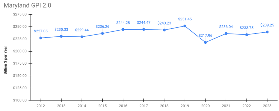
Maryland GPI
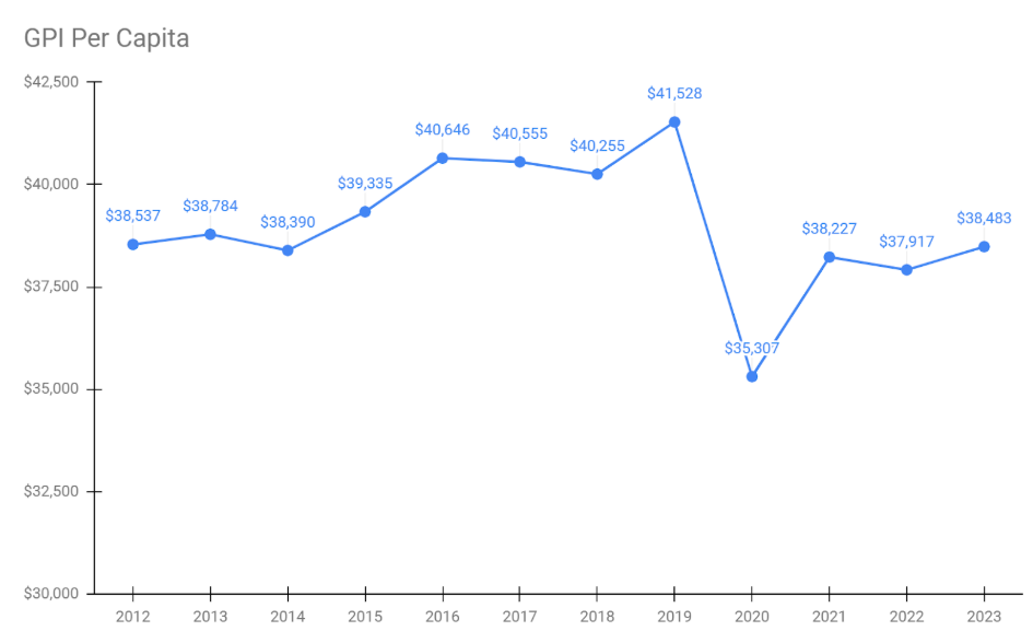
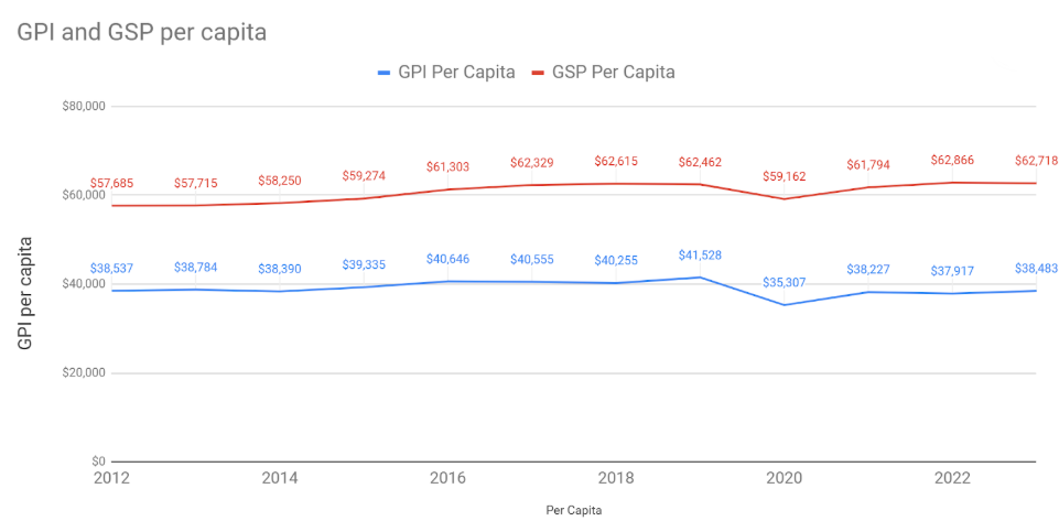
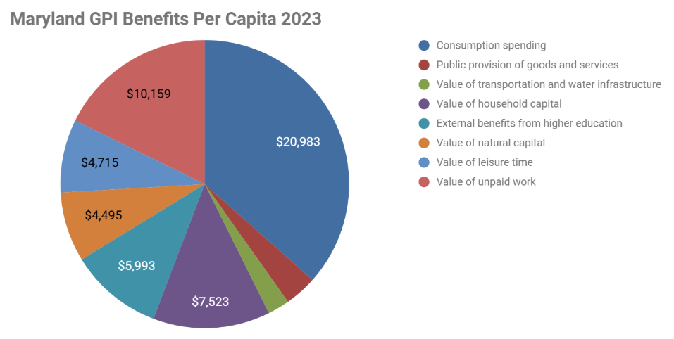
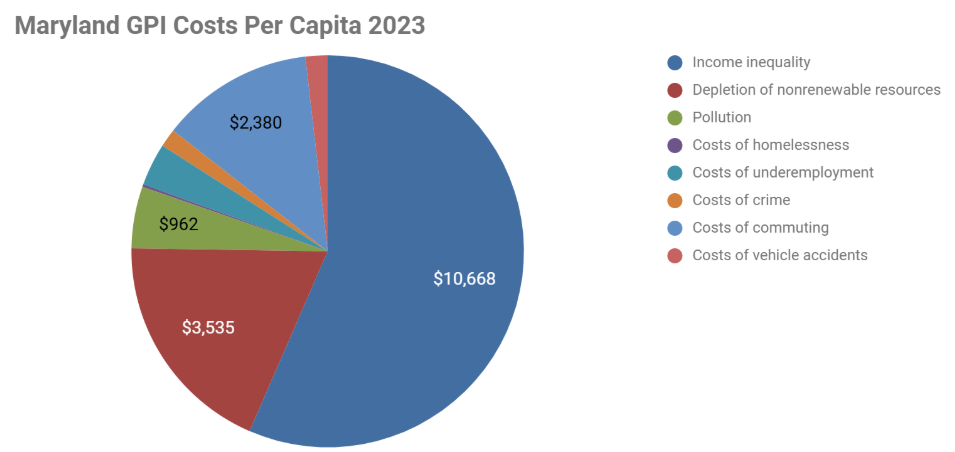
GPI per Capita
Trends in the Genuine Progress Indicator
2012 to 2023
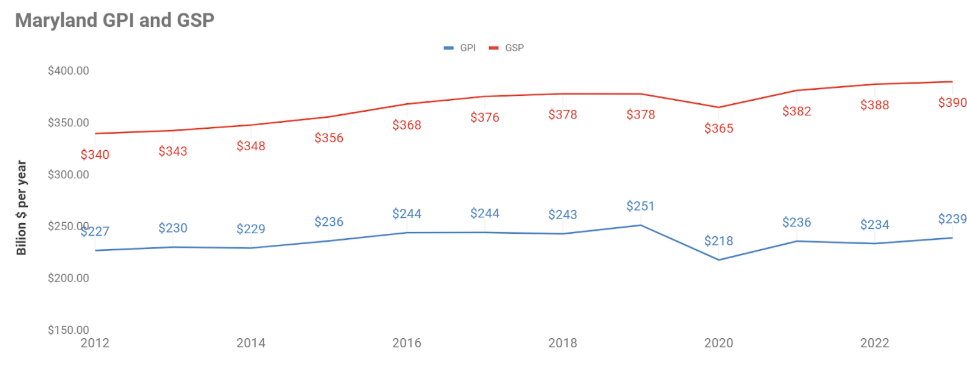
Overall the GPI increased by $12.2 billion over this 1210 year period, representing a 5.4% increase. In comparison, the Gross State Product of Maryland rose by $50.5 billion, or 14.7%, over this same period (normalized for inflation).
Household spending has increased 13.4% over the 12 year period but this has been offset by the increases in income inequality, defensive expenditures, and household investments. Non-market based well being increased over 15%, driven by benefits from higher education and unpaid labor, services from natural capital held steady. Environmental and social costs decreased by 13.5%. Within this category depletion of natural capital increased by nearly $300 million or 1.3%, due to loss of natural lands valued at $1.6 billion, which was offset by a 6.3% improvement in clean energy consumption. The cost of unemployment and underemployment declined by $7.3 billion or 63.8% since 2012, when unemployment rates still reflected lingering effects of the Great Recession.
2019 to 2020 – Impact of the Pandemic
The global coronavirus pandemic’s impact on society is reflected in the GPI indicators in several ways. Household budget expenditures fell by almost 5.7%, almost identical to the decrease in the gross state product from 2019 to 2020. However, this relatively small decrease belies the inequity in how the pandemic impacted people across income classes. The cost of inequality, which assesses the relative distribution of income, increased by 93% from 2019 to 2020. Unfortunately this increased disparity across income classes persisted through 2023. The 42% increase in low income food and nutrition assistance in 2020 also reflects the impact of the pandemic on lower income families. Other impacts can be seen in the decrease of library services and public art, music, and theater due to pandemic related closures, and the increase in subsistence hunting and fishing as these activities rose in popularity. The cost of underemployment increased tremendously, by 84%, while costs of greenhouse gas emissions and commuting fell due to fewer people being employed and the rise of teleworking options.
While some of these changes linked to the COVID pandemic had longer lasting impacts, overall the GPI, and GSP, returned quickly to prior levels in 2021.
Comparison of GPI 2.0 and 1.0 Results
Results are similar in trend using both 1.0 and 2.0 methods, but 2.0 shows a slightly smaller increase year over year from 2012 to 2013 (2.40% vs. 2.70%). The ending GPI value using 2.0 methods is $11 billion more than GPI 1.0 due to the fact that GPI 2.0 includes additional positive inputs, such as ecosystem services, public provisioning government spending, and services from libraries and the internet. These outweigh the additional costs considered in 2.0 like homelessness, groundwater depletion, and additional air pollutants.
